Suppose you are faced with a 10-arm bandit. For each arm, it has a distribution of reward. Your goal is to get as much reward as possible. But the problem is, you do not know the distribution (mean, variance, etc.). Your only method is trial-and-error, i.e. learn by trying. Now, I think that I should first evaluate my action and then take it by strategy.
How to evaluate an action?
1. Action value method
I evaluate each action by compute its mean reward till now.
$$ Q_{n+1} = \frac{1}{n}\sum_{i=1}^{n}R_i $$
2. Incremental Method for stationary problems
It can be achieved by incrementation, so that I can choose
$$ Q_{n+1} = Q_{n} + \frac{1}{n} (R_n - Q_n) $$
It is an update of Q value. At the beginning, it encourages exploration; as we step forward, we assign less and less weight to the current reward.
3. Incremental Method for nonstationary problems
Method 2 is effective in stationary problem, i.e. environment (state-action-reward) stay fixed all the time. If there is a sudden change in environment, we should use Method 3, where $\alpha$ is the step size.
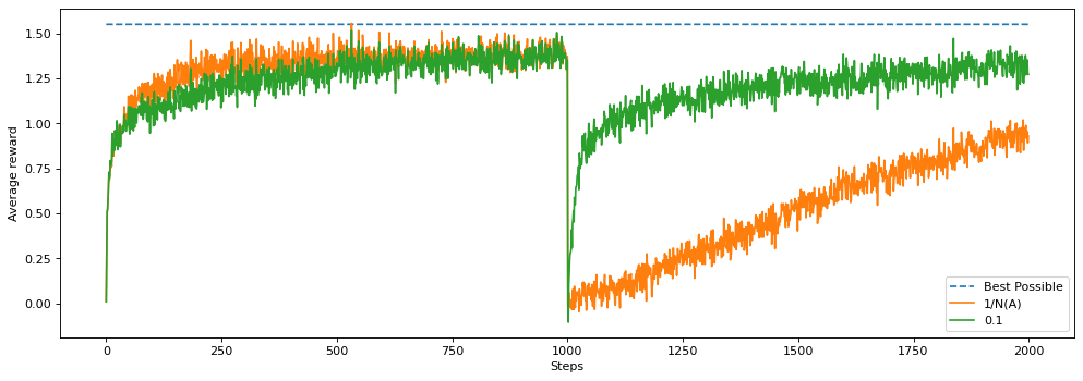 Step size is a trade-off between past and current. If $\alpha$ is larger, we are more adaptive to the environment change and quickly get to the true value. But it also makes q value senstive to environment. If $\alpha$ is small, it gets to the true value too slowly.
$$ Q_{n+1} = Q_{n} + \alpha (R_n - Q_n) = (1-\alpha)^n Q1 + \sum_{i=1}^{n}\alpha (1-\alpha)^{n-i} R_i $$ where $\alpha$ should satisfy $\sum_{n=1}^{\infty}a_n(a) = \infty$ and $\sum_{n=1}^{\infty}\alpha_n^2 (a) <\infty$
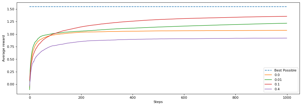
4. Optimistic Initial Values
Instead of zero initialization of Q, we set Q to a value (better if it is higher than all rewards). It can encourage exploration with the use of greedy policy. Imagine you set q to 4, and at the beginning, rewards is all below 4 for each action, so q is negative. Then we will jump to other actions. However, it only works well in stationary problem since it is a temporary drive for exploration.
How to take an action?
It is a problem of “policy” given q value. We often need to balance exploration and exploitation.
greedy action
take the action that leads to best q
def greedy(q_values):

    top_value = float("-inf")
    ties = []

    for i in range(len(q_values)):
        # if a value in q_values is greater than the highest value update top and reset ties to zero
        if q_values[i] > top_value:
            top_value=q_values[i]
            ties=[i]
        # if a value is equal to top value add the index to ties
        elif q_values[i] == top_value:
            ties.append(i)
        # return a random selection from ties.
    return np.random.choice(ties)
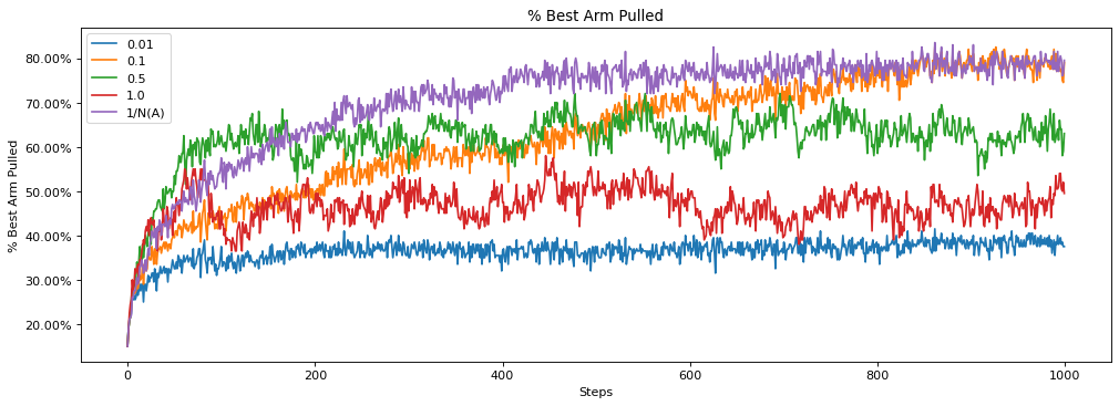
epsilon greedy
With probability $\epsilon$, take random action;
with $p=1-\epsilon$, take greedy action
def greedy(q_values):
     if np.random.random() < self.epsilon:
            # random
            current_action=np.random.randint(len(self.arm_count))
    else:
            current_action=greedy(self.q_values)


    return current_action
We need to choose an optimal parameter. 0.1 is a good value.
Upper-Confidence-Bound action selection
The intuition behind this method is we want to select actions with the highest upper bound of confidence interval.
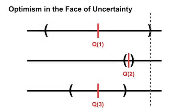 (from Coursera Fundamental of RL (Upper-Confidence Bound (UCB) Action Selection)
So we need to compute $mean + \frac{1}{2}confidence interval$. However, we do not know the distribution. So we should estimate upper confidence bound using the formula:
(from Coursera Fundamental of RL (Upper-Confidence Bound (UCB) Action Selection)
So we need to compute $mean + \frac{1}{2}confidence interval$. However, we do not know the distribution. So we should estimate upper confidence bound using the formula:
$$ A_t = argmax_a [Q_t(a) + c \sqrt{\frac{\ln t}{N_t(a)}}] $$ where the first half is exploitation strategy, the second half is exploration startegy; $c$ will control the balance; $t$ is the number of trials you have done and $N_t(a)$ is the number of times you select the action a. When $N_{t}(a)$ increase, the uncertainty decreases; when t increase but N not change, the uncertainty increases.
Reference
Reinforcement Learning: An Introduction Chapter 2: 2.4,2.5,2.6
Coursera: Fundamental of RL