Before we delve into solving MDP by dynamic programming, let’s review concepts in MDP!
Markov Decision Process
We can use MDP to describe our problems. It includes Action, State, Reward.
Markov Property
The next state could be fully derived by only the current state. $$P(s_t,r_t|s_{t-1}, a_{t-1}, \dots s_0) = P(s_t,r_t|s_{t-1},a_{t-1})$$
Reward Hypothesis
What we mean by goals and purposes can be well thought of as maximization of the expected value of the cumulative sum of a received scalar signal (reward). Sutton
Reward could come from the environment.
- goal-reward representation: 1 for goal, 0 otherwise
- action-penalty representation: 1 for not goal, 0 once goal reached
action-penalty representation could encourage early finding of goals.
- active research questions:
- How represent risk-sensitive behavior?
- How capture diversity in behaviors?
- Good matching for high-level human behaviors? ( create reward functions for ourselves? )
Valid policy
A valid policy is a conditional distribution of actions over states. That is, given the fixed state, you should act with probability. policy fliping action, like “L,R,L,R…” is not valid, cuz it depends on the last action. But if we include the last action to state, it is valid.
optimal policy
An optimal policy is defined as the policy with the highest value possible value function for all states. At least one optimal policy always exists, but there may be more than one.
Dynamic Programming
Policy evaluation is to evaluate the value functions of a policy. Policy control is to improve the policy. Since we have dynamics of the model $P$, we can use Dynamic programming to find the true value function and do improvement.
Value function and Bellman equation
We have defined the value function for each states if we follow the policy $\pi$ as the expected return: $$ v_{\pi}(s) = E_{\pi}[G_t|S_t = s] = E_{\pi}[\sum_{k=0}^{\infty} \sigma^k R_{t+k+1}|S_t = s]$$
The state-value function for policy $\pi$ is: $$q_{\pi}(s,a)=E_{\pi}[G_t|S_t = s,A_t=a]=E_{\pi}[\sum_{k=0}^{\infty} \sigma^k R_{t+k+1}|S_t = s,A_t=a]$$
There are recursive properties for value function and state-action functions. We will encounter them many times afterwards. The Bellman equation for $v_{\pi}$ is: $$ v_{\pi}(s) = \sum_a \pi(a|s) \sum_{r,s’} p(r,s’|s,a)(r+\sigma v_{\pi}(s’)) $$ for all s $\in$ S
The Bellman equation for $q_{\pi}$ is:
$$ q_{\pi}(s,a) = \sum_{r,s’} p(r,s’|s,a)(r+\sigma \sum_{a’} \pi(a’|s’) q_{\pi}(s’,a’)) $$ for all s,a $\in$ S,A
To get more reward as possible, we want to find the optimal policy $\pi*$ (maybe many) and they share one optimal value function and state-action function. They also have recursive properties. They are called Bellman optimality equations. $$q*(s,a) = max_{\pi}q_{\pi}(s,a)=\pi(a|s) \sum_{r,s’} p(r,s’|s,a)(r+\sigma max_{a’} q*(s’,a’))$$
$$v*(s ) = max_{\pi}v_{\pi}(s)=max_{a} \sum_{r,s’} p(r,s’|s,a)(r+\sigma v*(s’))$$
Our goal is to find solutions so we can use greedy action to behave the best!
It is a equation system with n state(unknowns) and n equations. So we can solve it by hand or using a solver. We can only do this under the condition that
- dynamics of the environment is known
- computational resources are sufficient to complete the computation (so not feasible for large models)
- the states have the Markov property
Now we are ready to see what we can do with DP! In general, it’s a method to iteratively or recurisvely achieve the result by dividing and reusing the problem.
Policy evalutaion
We define the value function at $k$ iteration as $v_k(s)$ for each state.
$$ v_{\pi,k+1}(s) = \sum_a \pi(a|s) \sum_{r,s’} p(r,s’|s,a)(r+\sigma v_{\pi,k}(s’)) $$
When $v_{k,\pi}$ achieves the true value function, it will not change.
Algorithm Input $\pi$
V = 0
V^ = 0
while True:
    diff = 0
    for s in S:
        V^(s) =  \sum_a \pi(a|s) \sum_{r,s'} p(r,s'|s,a)(r+\sigma V(s'))
        diff = max(diff, |V^(s)-V(s)|)
    V = V^
until diff < theta
Policy improvement
Policy improvement theorem: if $$ q_{\pi}(s,\pi’(s)) \geq q_{\pi}(s,\pi(s)) $$ for all s $\in$ S then $\pi’ \geq \pi$
if $$ q_{\pi}(s,\pi’(s)) > q_{\pi}(s,\pi(s)) $$ for all s $\in$ S then $\pi’ > \pi$
So if we improve policy by: $$ \pi’(s) = argmax_a \sum_{r,s’} p(s’,r|s,a) (r+\sigma v(s)) $$ we can find a strictly better policy $\pi’$ than $\pi$
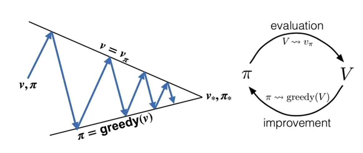
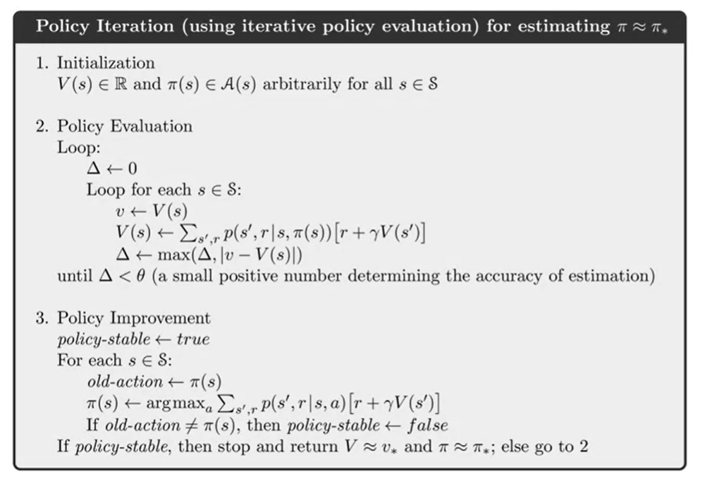
Policy iteration
We bounce back and forth between policy evaluation and improvement until the policy is stable.
Algorithm
Generalized Policy iteration
It’s a general idea of letting policy evaluation and improvement iteract, regardless of granularity and details.
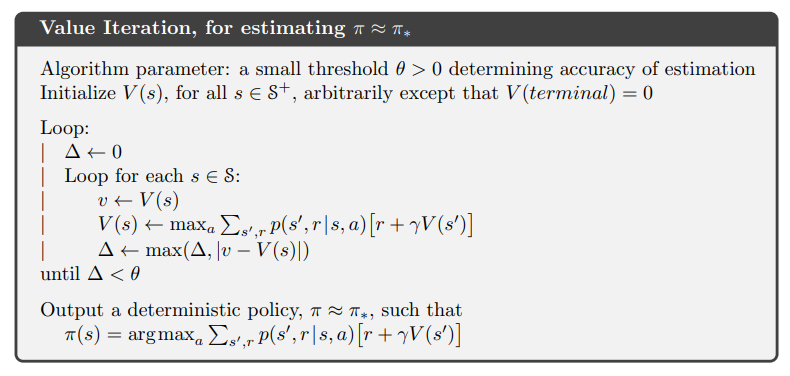
Value iteration
We can understand this as updating to compute Bellman optimality equation. It combines policy evaluation and improvement.
$$ v_{\pi,k+1}(s) = max_a\sum_{r,s’} p(r,s’|s,a)(r+\sigma v_{\pi,k}(s’)) $$
Asynchronous DP
It’s a DP that do not update systematically, but in any order. But it needs to update all states.
Alternatives to DP
Monte Carlo Method sample a lot of sequences, and compute the mean $$ v(s) = E(G|s) $$
Brute Force Search policy space to find the best one. Very time and space cost: $|A|^s$ Dynamic Programming
DP use Bootstrapping to improve efficiency. Bootstrapping use the other states we compute to compute the current state value function.
Better than Monte Carlo Brute Force, but also encounter problems with exponentially many states.