This is my final project of the class EIE3510 Signal Processing. I compare two traditional method and one deep learning methods. It’s a great journey to work with music!
Code: Music Source separation
Presentation: Music Source separation
Report
Introduction
The project aims to deal with a classical signal processing problem – music source separation. Specifically, separate the lead and the accompaniment in a song. In the project, I use music dataset MUSDB18HD, which contains 150 songs with different styles. Traditional methods (e.g. Sinusoidal model, REPET algorithm) and deep learning based method (e.g. Mask Inference) are applied. To quantitively measure the performance, I use evaluation metrics in Blind Source Separation (BSS), including Scaled Invariant Signal to Distortion ratio (SI-SDR), Signal to Artifacts ratio (SI-SAR), Signal to Interference ratio (SI-SIR). The deep learning method achieves the highest objective score. However, the result produced by REPET algorithm has the best sound effect. I mainly refer to the book \cite{opensourceseparation:book} to implement the algorithms.The demo and code will be available in the github repository.
Problem
Given a clean mixture signal, we expect the lead signal and accompaniment signals. We assumes a linear mixture of the lead and accompaniment model as follows: $$ z[n] = x[n] + \sum_{i=0}^{N-1}y_i[n] $$ where $z[n]$ is the mixture signal; $x[n]$ denotes the lead; $y = \sum_{i=0}^{N-1}y_i[n]$ represents the sum of multiple musical instrument tracks.
Approach
The frame of separating music sources could be depicted as Figure 1. Firstly, represent the signal in a form such that the sources are separable. The most common approach is the Time-Frequency representation, which could be obtained by Short Time Fourier Transform in \ref{sec:STFT}. The second stage is to detecting the assumed model in the TF representation, e.g. repetition pattern. The detected model and residual will be extracted by masking or filtering. Finally, the output signals will be transformed from frequency domain to time domain.
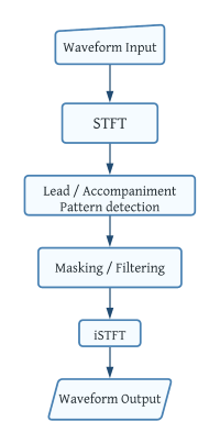 Figure 1
Short Time Fourier Transform
An STFT is computed by Discrete Fourier Transform (DFT) of the signal in a small window. We denotes $X[k,m]$ as DFT of the short part that starts at sample $m$, windowed by a window of length less than or equal to $N$ samples at frequency $w_k = \frac{2\pi k}{N}$ $$ X[k,m] = \sum_n x[n]w[n-m]e^{-jw_k(n-m)}, w_k = \frac{2\pi k}{N} $$ The $X[k,m]$ is put in the Time-Frequency matrix x at ($m,k$). $X[k,m]$ is complex number, but we usually use the absolute value of the real part to construct the magnitude spectrogram.
Model and Separation Method
To separate the lead and the accompaniment, the traditional methods usually construct a model based on some assumptions of the signals. Then, a series of transformations and masking will be applied to isolate signal sources. The traditional methods are model-based. I choose sinusoidal model, repetition model and harmoic-percussive model to analyze the mixture signals. Another stream of source separation method is driven by data, including methods in machine learning and deep learning. In the project, I use the mask inference method to train a mask, which extracts the vocals in spectrogram.
Sinusoidal Model and Analysis-Synthesis Method
The sinusoidal model assumes that the vocals are mostly harmonic, so they could be represented by a set of harmonics with fundamental frequency $\frac{2\pi k_0}{N}$.
$$ x[n] = \sum_{r=1}^{R} A_r cos(\frac{2\pi k_0 n}{N}) $$ $$ X_r[k] = A_r \sum w[n] \frac{1}{2}(e^{\frac{j2\pi r k_0 n}{N} + e^{-\frac{j2\pi r k_0 n}{N}}} e^{\frac{j2\pi r k n}{N}} $$ where x[n] denotes that the leads could be modeled as the sum of sinusoidal functions with different amplitude and related frequency; $X_r[k]$ is the DFT of each sinusoidal function.
Pitch Detection
One of the most commonly used pitch detection method is Autocorrelation. After computing the autocorrelation of a signal, the inverse of the point index with maximum ACF are regarded as the fundamental frequency of the signal. In this project, I use the Yin Algorithm in sonic visualizer to find the fundamental frequency of music in windows.
Separation
To separate the leads and the accompaniment, we need to identify the fundamental frequency in the song by pitch detection algorithms. Then we reconstruct the set of harmonics in spectral domains whose frequencies are integer multiplications of the fundamental frequency and whose amplitudes are the spectral envelope of the recording. The estimated vocal spectrogram is then converted to waveform.
Repetition Model and REPET algorithm
The accompaniment in the background are assumed to have repetitions, so that the structure could be extracted and exploited to separate the sources.
REpeating Pattern Extraction Technique (REPET)
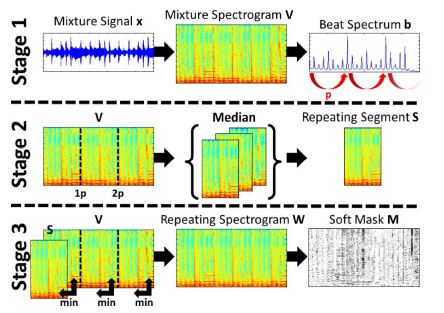
- Transform mixture signal from waveform $x$ to spectrogram $V$ and beat spectrum $b$. Find the fundamental repetition period $p$ in beat spectrum
- Divide $V$ into frame according to period $p$; take the median of frame as Repeating Segment $S$
- Compare each frame with $S$ and take the minimum value element by element; construct a Repeating Spectrogram $W$
- Compute Soft Mask $M$ as the $M = \frac{W}{V}$
Harmonic Percussive Source Separation algorithms
Combining two assumptions above, Harmonic Percussive Source Separation algorithm could extract the harmonic components and repetition pattern from original mixture. Harmonic Percussive Source Separation (HPSS) is derived accordingly.
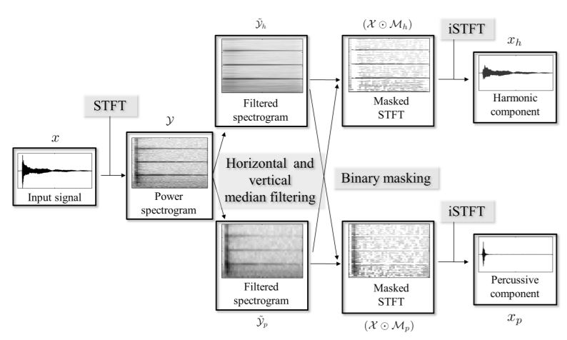
- Transform input signal $x$ to power spectrogram $y$
- Construct Filtered spectrogram by applying horizontal and vertical median filtering. Given a matrix $B \in R^{M\times K}$, the harmonic and vertical median filter are as follows: $$ medfilt_h(B)(m,k) = median(B(m-l_h,k),\dots,B(m+l_h,k)) $$ $$ medfilt_v(B)(m,k) = median(B(m,k-l_v),\dots,B(m,k+l_v)) $$ We get the enhanced spectrogram $y_h = medianfilt_h(y)$ and $y_p=medianfilt_v(y)$ respectively.
- Compute binary mask for harmonic and vertical components. Each point (m,k) in the mask are as follows:

Mask the magnitude spectrogram $X$ by $X \cdot M_h$ and $X \cdot M_p$
- Compute harmonic component $x_h$ and percussive component $x_p$ by inverse STFT
The harmonic and vertical median filter could enhance the horizontal and vertical features of the signals. The enhancement could extract the corresponding pattern out.
Deep Mask Inference
Suppose there exists an ideal mask which could extract the vocal components in the spectrogram as shown in the Figure 4. With help of deep learning, I train the model to learn such a mask.
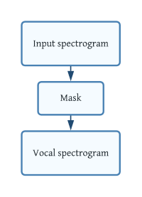 Figure 4
Architecture
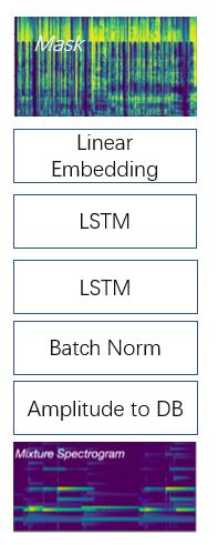
The neural network is composed of a batch normalization, two layers of LSTM, and a linear embedding, as depicted in Figure 5. The input and output size are the same $1724 \times 256$. The amplitude to DB layer will compute $10log_10(x)$ could improve the training via scaling. The LSTM layer with dropout rate 0.3 could do nonlinear transform on the input signal. The feature number in hidden layer of LSTM is 50, so the output size of LSTM is $1724 \times 100$. The linear embedding layer could map 100 features to 256 features.
Loss function
Suppose given the target source $Y$, trained mask $\hat{M}$ and the mixture spectrogram $X$, we estimate the vocals by $\hat{Y}=M \cdot X$. The L1 loss function is: $$ L=||Y-\hat{Y}|| $$
Training and testing
- Training data: 100
- Testing data: 500
- item Optimizer: Adam
- item Learning rate: 1e-3
Dataset
MUSDB18 is dataset of 150 full tracks. Each songs is consist of 4 source, vocals, drums, bass, and others. All signals are stereophonic and encoded at frequency 44.1kHz. For convenience, I use 30s of each track to process. In deep learning method, I use 100 data to train the model. In the testing stage, 50 pieces of music are used to evaluate the performance for all the algorithms.
Tools
I use sonic visualizer to visualize the spectrogram and analysis the music structure. For separation algorithms, I program in Python and exploit a signal processing package nussl.
Evaluation Metrics
According to \cite{roux2018sdr}, the SI-SDR, SI-SAR and SI-SIR are more robust metrics compared with SDR, SAR and SIR. Suppose a mixture $x = s+n \in R^{L}$, we estimate target source $s$ by $\hat{s}$. We can decompose the $\hat{s}$ to $e_{target} + e_{residual}$, leading to SI-SDR:
$$ SI-SDR = 10 log_{10}(\frac{|e_{target}|^2}{|e_{residual}|^2}) = 10 log_{10}(\frac{|\frac{\hat{s}^{T}s}{|s|^2}s|^2}{|\frac{\hat{s}^{T}s}{|s|^2}s-s|^2}) $$
The $e_{residual}$ could be further decomposed to $e_{interference}+e_{artifacts}$. The $e_{interference}$ is the projection of $e_{res}$ into subspace spanned both by s and n. The SI-SIR and SI-SAR are defined as follows:
$$ SI-SIR = 10 log_{10}(\frac{|e_{target}|^2}{|e_{interference}|^2}) $$ $$ SI-SAR = 10 log_{10}(\frac{|e_{target}|^2}{|e_{artifact}|^2}) $$
Result
I use a song from The Beatles. The waveform and spectrograms are shown in Figure 6. In the testing, I use the first song in test set as an example.
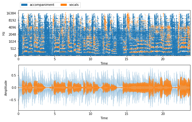 Figure 6
Music Structure Analysis
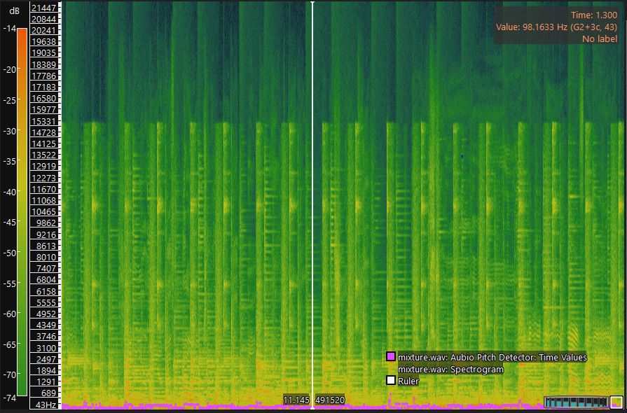
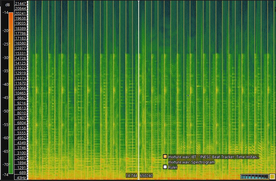
I use window size 1024. In Figure 7, the pink line represents the pitch detected. Pitch varies from 98Hz to 300 Hz. In Figure 8, the orange line represents the detected beat. The fundamental beat period is 0.546s.
Separation
The following figures are the spectrogram and waveforms of the estimated vocals as well as accompaniments for the Beatles’ song.
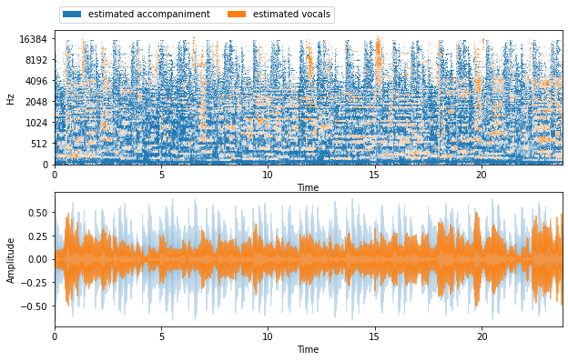 Figure 9
Please kindly note that the color in HPSS result is reverse of others.
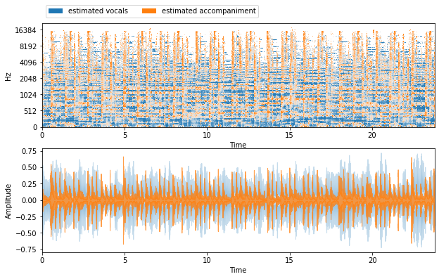 Figure 10
REPET
The REPET algorithm have a relatively good performance.
 Figure 11
HPSS
Please kindly note that the color in HPSS result is reverse of others.
 Figure 12
Deep Mask Inference
The training loss is depicted as follows.
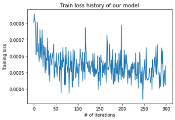 Figure 13
The result of separation for the Beatles’ song in the training dataset.
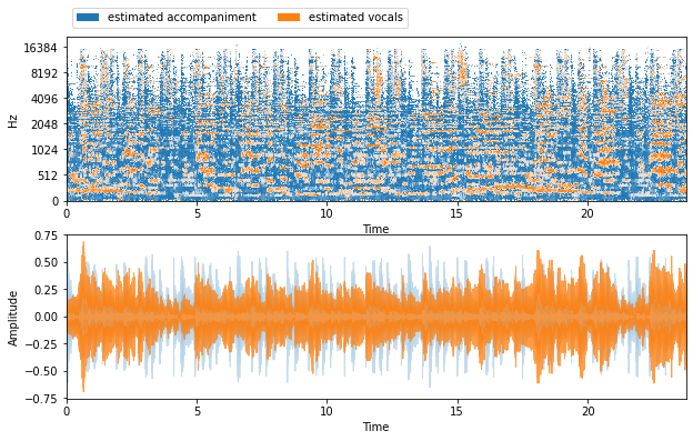 Figure 14
Testing
In the testing set, I compare the four methods via subjective and objective measure on 50 data. The results are median of the metrics. While REPET has the best sound effect, the deep learning method get highest scores in the objective measure. The gap may be due to the nature of music. We evaluate the music by hearing it. There are some critical features in music, which could make a big difference in sound effect via a tiny fluctuation in number. Therefore, the subjective and objective measure could not accord with each other.
Another problem of all methods is that the vocals are mixed with the guitar melody. Two traditional methods assumes the accompaniments have repetition patterns. The assumption work well for the drums, but they could not be generalized to the accompaniments with melodies. For deep learning method, it could extract the common features of all songs, repetition. However, the guitar accompaniment does not have a fixed pattern in spectrogram, since every song has different harmonics. To solve the problem, more complex model for accompaniment (e.g. low rank assumption) should be exploited.
 Figure 15
Conclusion
In the project, I use sinusoidal model, repetition model, harmoic-percussive model and Deep Mask Inference to solve the lead-accompaniment problem. The analysis and separation methods have sound performance in separating drums and vocals, but the music instrument with melodies could not be extracted. Although deep learning method have highest objective scores, it suffers from the variation of music so the sound effect is not up to expectation. Through this project, I have a basic understanding of the music source separation problem. I also learn different models regarding the leads and accompaniments. The programming implementation deepens my understanding various solutions to the problem.